Main Menu

Chapter 3 Slides(pptx)

Errata

Last updated 2019-10-08

1. p. 34 modified note 3 adding a reference which describes one of Young’s experiments.
2. p. 38 line 11 should be “replace 1/r1,2 with their average”
3. p. 41 Example 3.3 the extra e^ikz on the 2nd line of the equation should not be there.
4. p. 45 Fig. 3.18 x and z should be swapped in Figure.
5. p. 46 Note 19: R in two equations replace with calligraphic R.
6. p. 47 Fig. 3.20 labels in plot inconsistent with axis scale which is phase over 2 pi. Added extra Example.
7. p. 48 add side note to clarity 1/2 factor in equation.

Exercises

1. (3.3) r should be r’ to be consistent with notation in Chapter. Final sentence should be “in order [to] re-write….”

Extras

Thin-film interference: white light

Topics: Interferometry, white light

Optics textbooks tend to be rather monochrome. When we plot Young’s interferference fringes or diffraction patterns we tend to assume monochromatic light. However, some of the most interesting interference effects like soap films (see e.g. here and below) are observed using ‘white light’. In Chapter 8 of Optics f2f we discuss white light and in the Excercises include a plot of Young’s double-slit experiment using more than one wavelength (p. 146 in Optics f2f). Making colour plots of diffraction or interference phenomena raises some interesting issues that are not widely discussed. The purpose of this post is to illustrate the issues involved using another example – Newton’s rings. The image below (by James Keaveney) is an award-winning photograph of a Newton’s ring pattern produced when two pieces of quartz (one with a slight curvature) are placed almost touching and illuminated with white light. This amazing optical component was made by the brilliant David Sarkisyan and colleagues in Armenia, and is used to perform experiments on light-matter interactions in nanoscale geometries (see e.g. here).

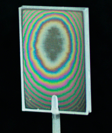
In the middle, where the separation between the two reflecting surface is less than the wavelength, we see darkness surrounded a white fringe, which in turn is surrounded coloured fringes. Moving away from the centre we only see one more darkish fringe before the interference pattern ‘washes out’, as expected for white light (see e.g. Figures 8.5, 8.6 and 8.15 in Optics f2f). We can model this assuming an intensity pattern of the form (see p. 41 in Optics f2f) I/I_0=sin^2[pi rho^2/(2 lambda R)], where rho is the distance from the centre, lambda is the wavelength and R is the radius of curvature of one surface. To model white light we simple add together the intensity patterns for each wavelength. But this is where it gets tricky. The spectrum of sunlight (shown below, data from here) and most other ‘white-light’ sources is complex (e.g. the narrow dips in the solar spectrum are the famous Fraunhofer lines).

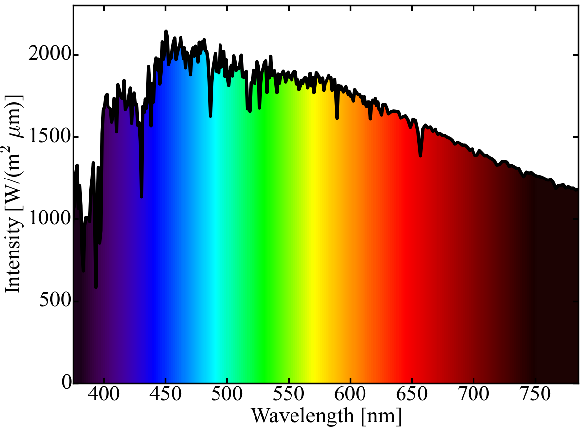
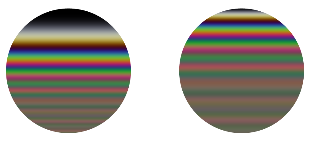
In principle, we could simulate sunlight interference by sampling the intensity at say 1 nm intervals between 400 and 650 nm and then summing the resulting 250 intensity patterns but this is computationally rather intensity. Alternatively, we could try to exploit the fact that the eye and colour image sensors only measure 3 colour channels, R, G, and B. So, is it sufficient to reproduce the pattern by summing only 3 intensity patterns corresponding to the red, green, and blue channels? The answer is no. Although, at first this may seem surprising, the reason why should be apparent to students of Optics f2f). Adding the intensity patterns for different colour is about adding waves with different spatial frequency and we learn from Fourier that a discrete spectrum is not great at reproducing and continuous spectrum. We see this perferectly in e.g. Figures 8.5 of Optics f2f) where we see that the interference pattern for 5 colour channels on row (iv) does not gives the same result as the continous spectrum on row (v), although the approximation is not bad for small path differences. To you and me the right mix of RGB (what photographers would call white balance) looks like white light and we cannot tell the difference between a discrete and a continuous spectrum until we do interferometry (oil films or soap bubbles are probably the most familiar examples). So coming back to Newton’s rings. First, I show the pattern calculated for three discrete colours (an R, G, and B channel only). As a source this looks like white light but if we look at the Newton’s ring pattern it looks very different to the James Keaveney photo.

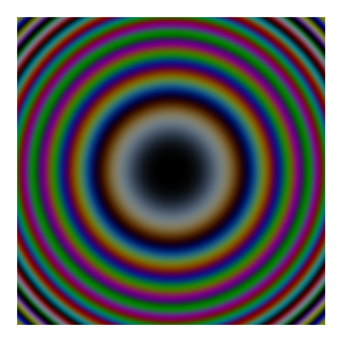
In particular, we see different colours (yellow) and a repeat of the dark fringes towards the edges of the pattern. Now if we increase the number of wavelengths to 12 we get this.

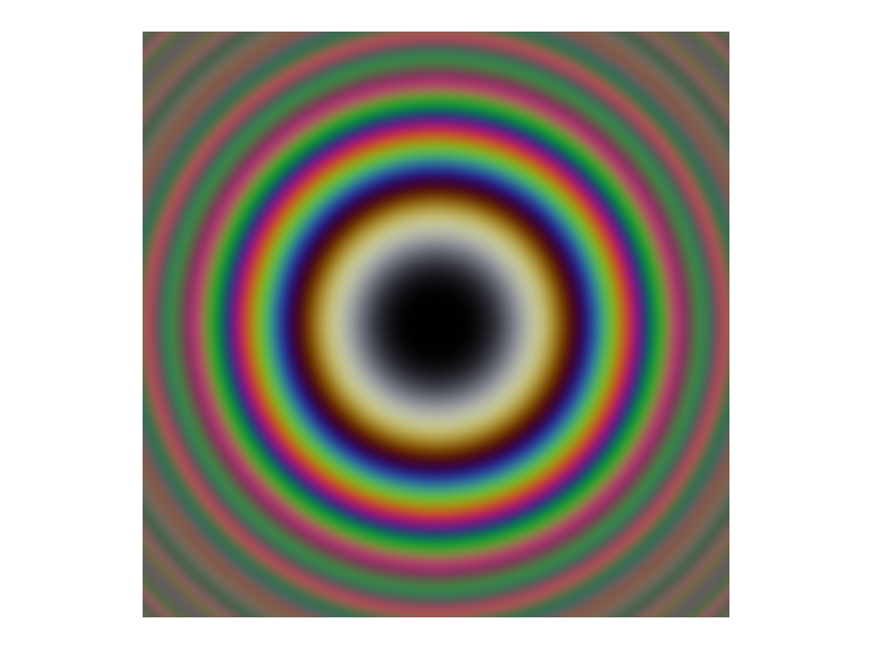
This is much closer to the photo and in my subjective view is a reasonable approximation to case of continuum white-light illumination. In particular, we see how the intensity fringes ‘wash out’ as we move away from the centre, like in the photo. However, as we are still using a discrete spectrum, if we extended the image further we would again see a repeat of the dark fringes. As Fourier taught us, only a continuous spectrum will suppress all repeats of the pattern. Now to make the 12 wavelength image we have to decide on a wavelength to RGB mapping. Wavelength to RGB conversion is used to create the colour in the solar spectrum plot above. Exactly how this is done is somewhat subjective (an example is given here). Bascially we are free to play around with the map untike we like the result (similar to how a photographer adjusts white balance in post-processing). Colour is a more of an art than a science which is perhaps why it is seldom covered in optics textbooks. Here is the python code to make the Newton’s rings pictures.

from numpy import linspace, sin, cos, shape, concatenate, dstack, pi, size
from pylab import figure, clf, show, imshow, meshgrid
from matplotlib.pyplot import close

X, Y = meshgrid(linspace(-0.85*pi,0.85*pi,500), linspace(1*-0.85*pi,1.0*0.85*pi,500))
R=0*X #initialise RGB arrays
G=0*X
B=0*X

#'''
wavelengths=linspace(0.4, 0.675, 12) # define 12 wavelengths + RGB conversion
rw=[0.1, 0.05, 0.0, 0.0, 0.0, 0.0, 0.0, 0.1, 0.13, 0.2, 0.2, 0.05]
gw=[0.0, 0.0, 0.0, 0.067, 0.133, 0.2, 0.2, 0.1, 0.067, 0.0, 0.0, 0.0]
bw=[0.1, 0.15, 0.2, 0.133, 0.067, 0.0, 0.0, 0.0, 0.0, 0.0, 0.0, 0.0]
#'''
'''
wavelengths=linspace(0.45, 0.6, 3) # define 3 wavelengths
rw=[0.0, 0.0, 0.5]
gw=[0.0, 0.5, 0.0]
bw=[0.5, 0.0, 0.0]
'''
num=size(wavelengths)

for ii in range (0,num): #add intensity patterns into the RGB channels
    field=sin((X*X+Y*Y)/wavelengths[ii])
    intensity=field*field
    R+=rw[ii]*intensity
    G+=gw[ii]*intensity
    B+=bw[ii]*intensity

RGB=dstack((R, G, B))

close("all")
fig = figure(1,facecolor='white')
clf()
ax = fig.add_axes([0.05, 0.05, 0.9, 0.9])
ax.axison = False
ax.imshow(RGB)
show()

Exersize: Finally, as an exercise, how does thickness vary with position in the two soap film pictures below?

Thin-film interference: Anti-reflection (AR) and high-reflectivity (HR) coatings

Topics: Interference, Fabry-Perot

In a wide variety of applications it is important to have an interface without undesirable reflections. This is achieved using an anti-reflection (AR) coating. Alternatively, we might want to reflect all the light with low loss, for example, inside a laser cavity. This is achieved using a high reflectivity (HR) coating. The mathematical description of AR and HR coatings is presented in the attached worksheet. The solutions are produced using a python notebook here.