Chapter 6 Slides(pptx)

Errata

Last updated 2019-10-08

p. 93. Mistake in equation (6.5), the coefficients of the complex Fourier series.
p.100 Add extra sidenote to remind reader of meaning of E^(z) and E^(0).
p.100 Include dy’ in first line of eqn (6.33). Second line E^(z) in integral changed to E^(O).
p. 45 Fig. 3.18 x and z should be swapped in Figure.
p. 46 Note 19: R in two equations replace with calligraphic R.
p. 47 Fig. 3.20 labels in plot inconsistent with axis scale which is phase over 2 pi. Added extra Example.
p. 48 add side note to clarity 1/2 factor in equation.

Exercises

(6.5) part (i). LHS of first equation should be f(x), not a_j.
(6.16) part (i). “the” added before “horizontal and vertical”

Extras

2D optical Fourier transform of an image

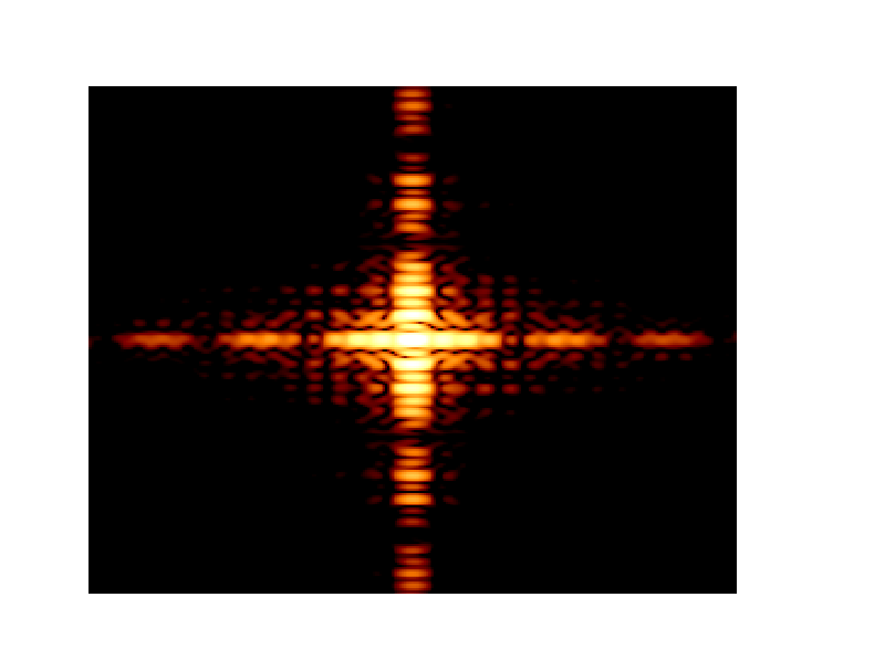
In Optics f2f we frequently use the example of letters to illustrate Fraunhofer diffraction (Chapter 6), convolution (Chapter 10 and Appendix B), spatial filtering (Chapter 10) and the properties of Fourier transforms in general (Chapters 6, 10 and Appendix B). Below, we share a python code, based on eqns (6.35) and (9.9) in Optics f2f, that calculates the intensity patterns associated with the optical Fourier transforms of letters. The code works by printing a letter as an image, e.g. an E

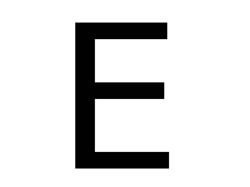
then digitising this image as an array, calculating the Fourier transform, and finally plotting the modulus squared as a colormap.

This code (last updated 2019-02-14 [1]) evaluates eqns (6.35) and (9.9) in Optics f2f for cases where the input aperture function has the shape of a letter.

from numpy import frombuffer, uint8, mean, shape, zeros, log, flipud, meshgrid
from numpy.fft import fft2, fftshift, ifftshift
from matplotlib import figure, cm
from matplotlib.pyplot import close, show, figure, pcolormesh

close("all")
fig = figure(1,facecolor='white')
ax = fig.add_axes([0.1, 0.1, 0.8, 0.8]) #add axis for letter
ax.axison = False
ax.text(-0.5,-1.0, 'Z', fontsize=460,family='sans-serif') #print letter
ax.set_xlim(-1.0,1.0)
ax.set_ylim(-1.0,1.0)

fig.canvas.draw() #extract data from figure
data = frombuffer(fig.canvas.tostring_rgb(), dtype=uint8)
data = data.reshape(fig.canvas.get_width_height()[::-1] + (3,))
bw=mean(data,-1)/255.0
bw-=1.0 #invert

[xpix, ypix]=shape(bw)
mul=4 # add zeros to increase resolution
num_x=mul*xpix
num_y=mul*ypix
H=zeros((num_x,num_y))
H[int((num_x-xpix)/2):int((num_x+xpix)/2),int((num_y-ypix)/2):int((num_y+ypix)/2)]+=bw
F=flipud(fftshift(fft2(H))) #perform Fourier transform and centre
Fr=F.real
Fi=F.imag
F2=Fr*Fr+Fi*Fi #calculate modulus squared
Fs=F2[int((num_x-xpix/2)/2):int((num_x+xpix/2)/2),int((num_y-ypix/2)/2):int((num_y+ypix/2)/2)]

fig = figure(2,facecolor='white')
ax = fig.add_axes([0.1, 0.1, 0.8, 0.8])
ax.axison = False
p=ax.pcolormesh(log(Fs),cmap=cm.afmhot) # plot log(intensity) pattern
p.set_clim(12,20) #choose limits to highlight desired region

show()

[1] Note, code works using python 2 and 3. Cut and paste text into jupyter notebook. Last tested using jupyter with python 3.7.1 numpy 1.15.4 and matplotlib 3.0.2.

Light propagation codes

Topics: angular spectrum, hedgehog equation, gaussian beams, split-step Fourier code.

Many of the figures in Optics f2f showing light propagation by solving the hedgehog equation, eqn (6.29) on p. 98. Here we present a basic light propagation code and show how to test it. The numerics are based on the split-step Fourier method, described on p. 99. In most examples, we will use only one transverse dimension, along x, and propagate the field along z. The final example considers the extension to two transverse dimensions. The idea is very simple, we take the Fourier transform of the input field, multiply by the propagator, exp(ik_zz), and then perform an inverse Fourier transform to find the output field a distance z downstream. A Fast Fourier Transform is included in most scientific software packages. To test our it code we need to compare it to something where we know the answer. A good example is the gaussian beam where the propagation is analytic so we can compare our numerical solution calculated using the hedgehog equation with the analytic results of Section 11.2. The python code here plots the intensity at the beam waist and at two positions downstream, see Figure 1. In the right hand column we plot the corresponding momentum distribution, which of course does not change because momentum is conserved. The discrete points (red and blue) show the output of the code and the lines show the analytic results. The actual propagation part of the code is only a few lines (beginning with the comment calculation angular spectrum) most of the rest is to make the plots. We recommend having a play with this code. In particular try varying the radius of the laser beam waist, w₀ (4th line down in the parameters section near the beginning of the code). Notice how if you double or halve the beam waist then the width of the momentum distribution halves or doubles, respectively, and the beam spreads out less (or more). This is Heisenberg’s uncertainty relation, eqn (6.26) and Fig. 6.8, in action.

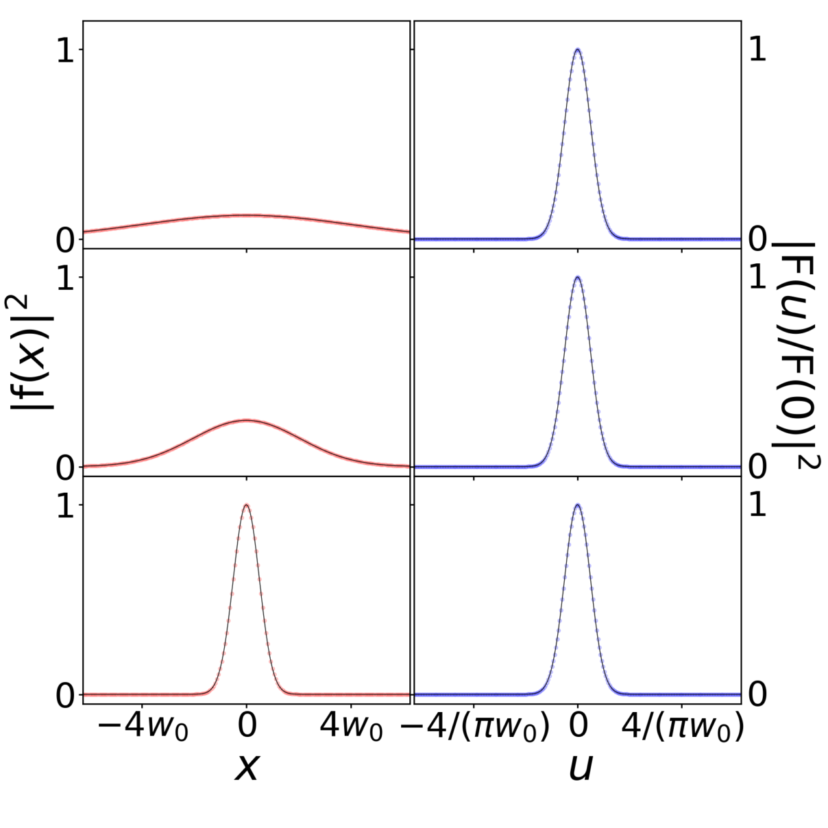
Figure 1: Test of angular spectrum propagation code for a gaussian input. The code (red and blue points) is compared to the analytic formulas for gaussian beam propagation (lines) taken from Section 11.2.

The other parameter to vary is the spatial resolution, dx. Importantly dx sets the maximum momentum included in the simulation, so if dx is too large then the momentum range may become too small. Try increasing dx by a factor of 16 to 4λ. For w₀ = 4λ, the code still does a reasonable job but now the range of momenta is only just sufficient. Another factor of 2 (dx = 8λ) and the code breaks as the momentum range is too small. This split-step Fourier code can be used as a basic building block for any light propagation simulation. The main limitation is the computation power required if you want to simulate a region with dimensions many times the wavelength, especially if two spatial dimensions are involved. Next we shall consider a number of examples to illustrate aspects of white-light propagation, focussing and two transverse dimensions (a circular aperture). Other examples can be found in Chapter 9 and 10 Extras.

White-light propagation

Topics: angular spectrum, hedgehog equation, gaussian beams, split-step Fourier code

It is easy to extend the split-step Fourier code to simulate different wavelengths. In fact, the only thing that changes is the propagator. There is some useful insight here that is easy to miss if we only consider monochromatic light. The tranverse momentum distribution of any light field ONLY depends the transverse spatial distribution. It does not depend on the wavelength. This is easiest to see for the example of a gaussian beam where we found that the transverse momementum width, Δp, is equal to ℏ/2 divided by the spatial width, Δx, in agreement with Heisenberg’s uncertainty relation. The spread of a gaussian is illustrated in Fig. 6.8 in Optics f2f. So the question is if the transverse momentum distribution is the same, why does red light (longer wavelength) diffract more than blue (shorter wavelength)? The answer is because the axial (or longitudinal) momentum is different. The angular spread, Δθ = 2Δp/p, see Fig. 6.8 caption. For a beam with a particular transverse width Δp is the same regardless of colour, but p changes. Red light has a smaller longitudinal momentum than blue and therefore if they both have the same transverse distibution red will spread out more than blue. This effect should appear in our propagation code when we simulate different wavelengths. The code here simualates the propagation of three overlapping laser beams, a red (at 633 nm) a green (at 520 nm) and a blue (at 450 nm) each with the same initial size, w₀. Each wavelength requires a different value of k in the propagator, exp[i(k²–k_x²)^1/2]. In the code we have chosen to scale our spatial dimensions in units of the green wavelength and then define k_red and k_blue in terms of k_green. Note that k_x, the Fourier variable, remains the same for each wavelength. Figure 2 shows the result when the three colours are overlapping and Figure 3 shows them separated. We can clearly see that red spreads out faster than blue, as would expect recalling the result that Δθ=λ/(λ w₀). This leads to the red fringing at the edges of the beam in Figure 2. We saw the same red fringing effect when we tried to focus red green and blue light, see Chapter 9 Extras.

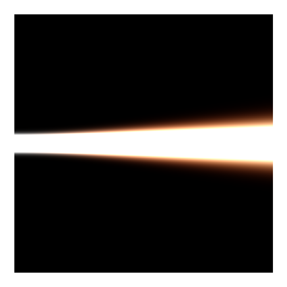
Figure 2: Test of angular spectrum propagation code for overlapping red, green, and blue laser beams with the same initial size. The red tinges on the right indicate that the red diffracts more than the blue.

In Figure 3 we repeat the same simulation but now with the three colour separated along the x (vertical) axis. This plot illustrates how red spreads (diffracts) out faster.

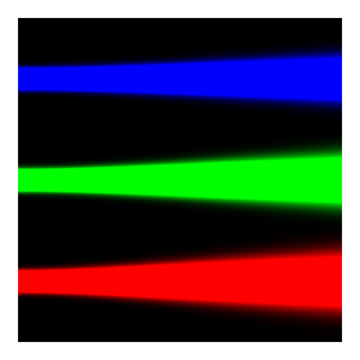
Figure 3: The same as Figure 2 except now with the three beam separated out to illustrate the faster angular divergence of longer wavelengths, Δθ = λ/(λ w₀).

Light propagation: refraction and dispersion

Topics: refraction, refractive index, Snell’s law, dispersion

One feature we might might to add to our angular spectrum code is how light propagates inside a medium. A simple ‘zero-order’ approximaion is to replace k by nk, where n is the refractive index. We call it ‘zero order’ because it does include the backwards propagating fields (see Chapter 13 in Optics f2f) or the vector property of the electric field (see Chapter 13 in Optics f2f). However, it does allow us to look at refractive and dispersion in simple structures with dimensions larger than the wavelength such as prisms and lenses. An important requirement for simulating an interface between media with different refractive index is that our spatial grid needs to be finer than the wavelength such than the interface looks ‘smooth’ on the scale of the wavelength. The code here models a quasi-white-light beam propagating through a prism as in Newton’s classic experiment or on the cover of Dark Side of the Moon. How could be album cover be improved?

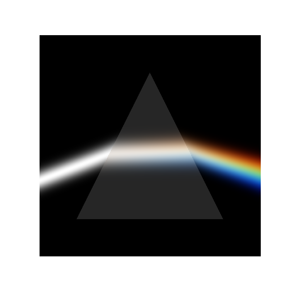
Figure 4: Refractive of ‘white’ light by a dispersive prism.

The code makes a refractive index ‘island’ in our xz space. Instead of an island with the shape of a prism, we can define a plano-convex shape to simulate a lens as in this code. Note that we are simulating a cylindical lens, as we are assuming the everything is uniform in the along y direction.

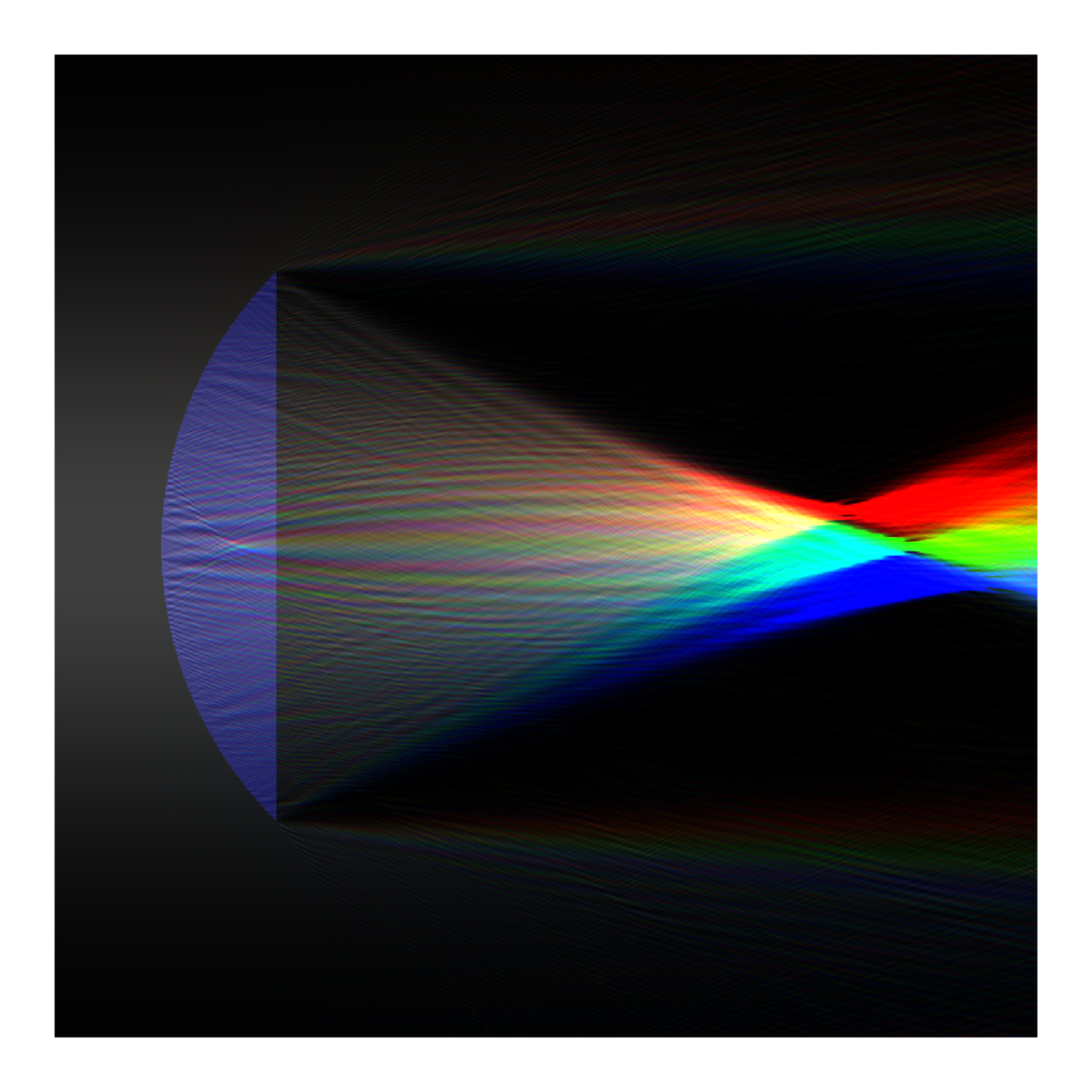
Figure 5: Pseudo-white light made of red, green and blue lasers propagating through a achromatic plano-convex lens, where achromatic in this case means that the refractive index is the same for each colour. The focal shift arises due to the different momenta of red and blue light.

The surprising result here is that even for an achromatic lens different colours focus in different planes due to diffraction. This effect, known as the focal shift, is discussed in relation to laser beam where we can derive an analytic result in Chapter 11, see Fig. 11.5 on p. 181. The focal shift is approximately the focal length cubed divided by the Rayleigh range of the input beam squared so is proportional to wavelength squared. It follows that the focal shift is larger for red light as we see in Figure 5. The focal shift is relatively large in this case because spatial extent of the simulation is small. In practical imaging examples where the distances involves are much larger the diffraction shift is usually much smaller than the dispersion shift (chromatic aberration). Have a play around with the code and see if you can compensate the diffraction focal shift with dispersion and then see what happens as you can the input beam size.

Light propagation: 2D transverse dimensions

Topics: angular spectrum, hedgehog equation, split-step Fourier code, Fresnel diffraction.

As a final example we consider the extension to two transverse spatial dimensions x and y. The main changes are to replace fft and ifft with fft2 and ifft2 as in this code, and the input is now a 2D array. The code plots the intensity in either the xz or the yz planes downstream of a circular aperture. We could also plot the field in any xy plane at a particular z with is less demanding as we only need to perform the Fourier transform and inverse transform once. The problem with 2D fft is that it quickly becomes computational intensive. For 400×400 points in the xy plane and 1000 slices in the propagation direction z this code takes about a minutes on a laptop with a i7 processor.

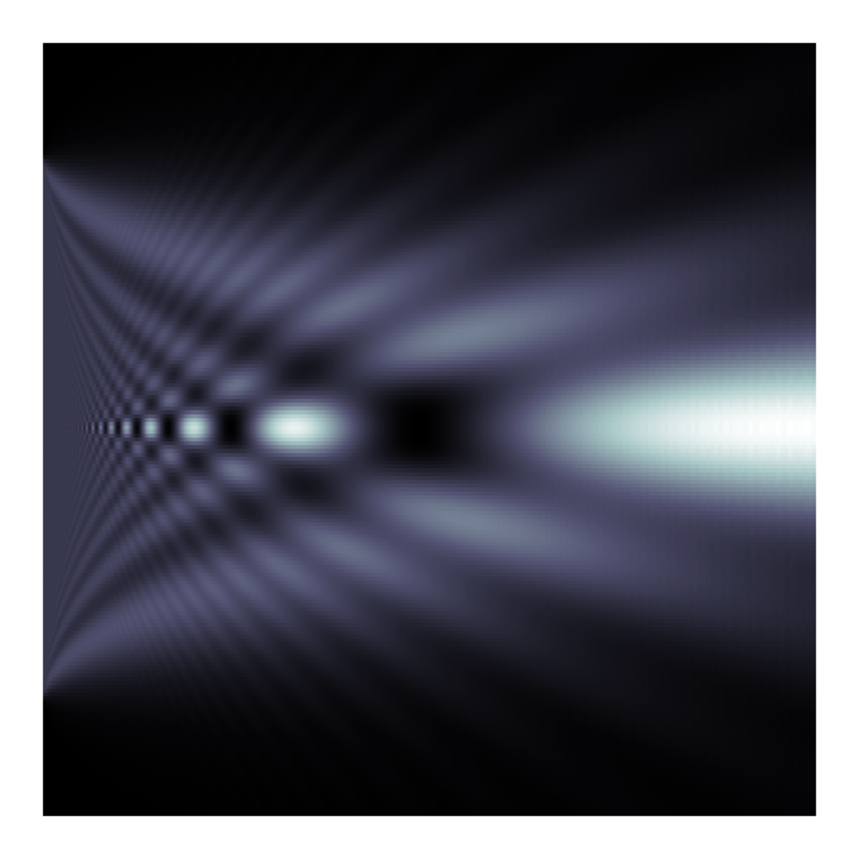
Figure 6: The intensity distrubution in the xz plane downstream of a cicular aperture. The light is propagating from left to right. The same as Figure 5.9(ii) on p. 79 of Optics f2f

For the case of a circular aperture it is possible to use an analytic solution involving a sum of Bessel functions. But there are many interesting problems where this is not the case and a 2D Fourier transform is the only option. The front cover of Optics f2f and Figure 7 which show the light field in the shadow behind two circular discs were produced using this code.

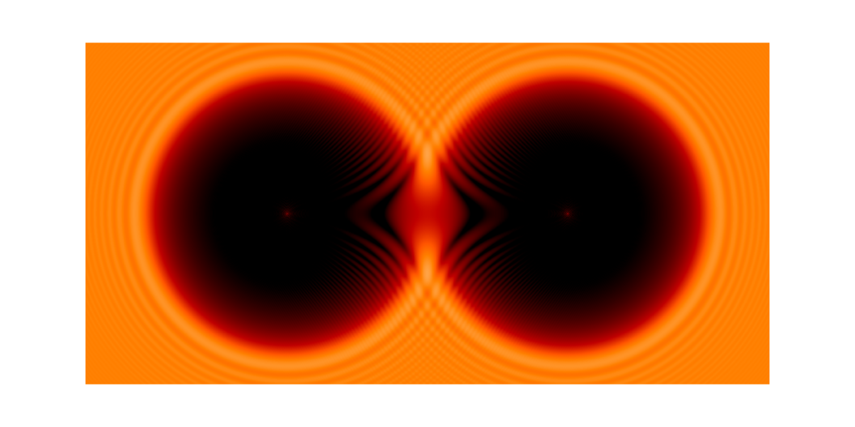
Figure 7: The intensity distrubution in the xy plane a distance z downstream of two circular discs (or two ball bearings see Fig. 5.1 in Optics f2f).