Chapter 5
Chapter 5 Slides(pptx)
Errata
Last updated 2019-10-08
- p. 72 remove 1/(ikz) from eqn (5.1) and define A immediately after.
- change “The phase of these contributions oscillates” to “The sign of these contributions oscillates” and “In Fig. 5.5 we have labelled two points …., where the phase changes sign.” to “In Fig. 5.5 we have labelled two points … where the field contributed changes sign.”
- p. 75 before eqn (5.9) condition should be f(rho’)=1 for rho’ less than 1, 0 otherwise.
- p. 83 Example 5.6. should be e^(-x^2/w_0^2) in integral. Eqn (5.35) delete (lambda z) in numerator of right hand equation.
Extras
From Fresnel to the lighthouse
Topics: Fresnel diffraction, Circular aperture, Fresnel zones, Fresnel lens
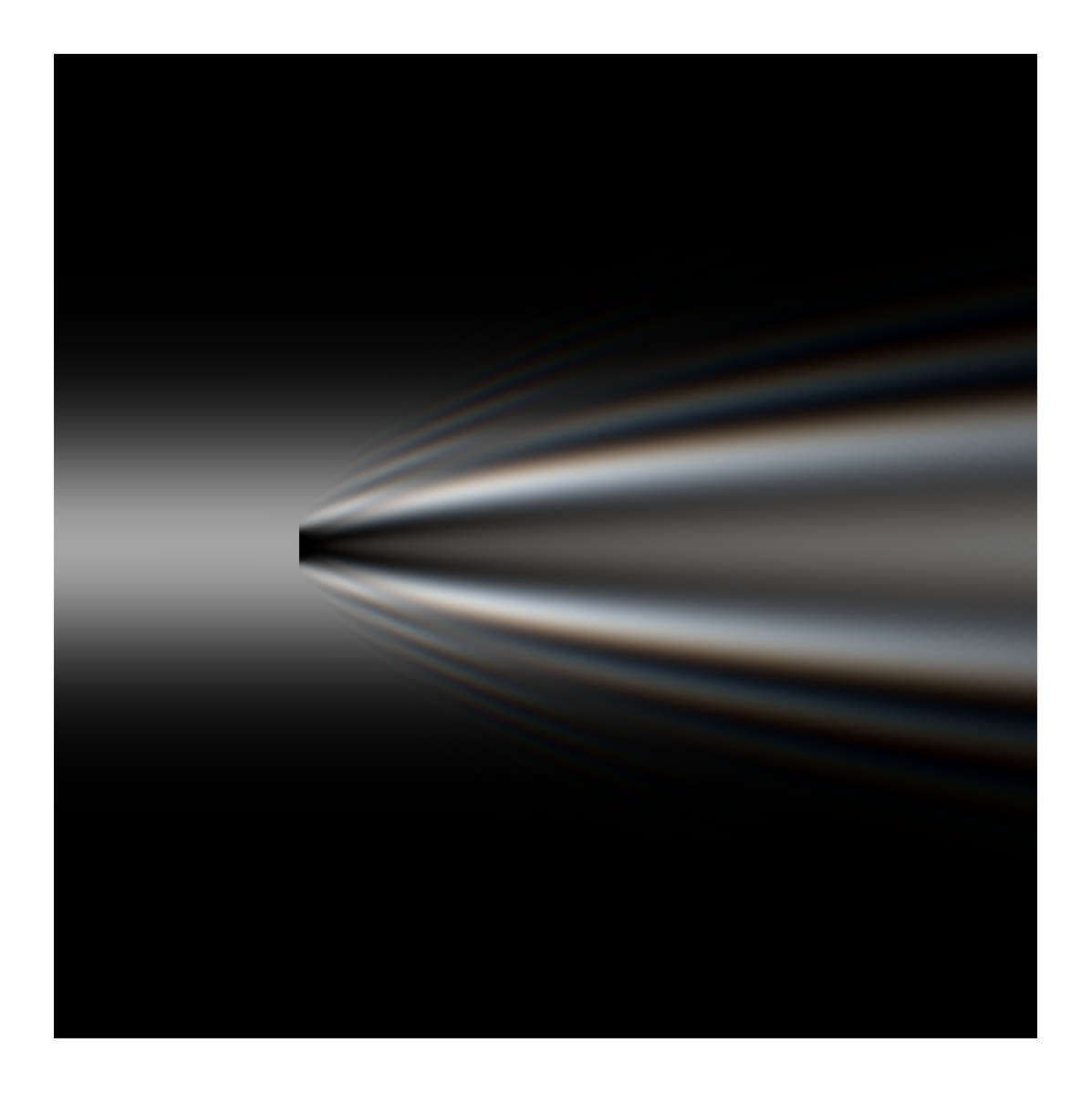
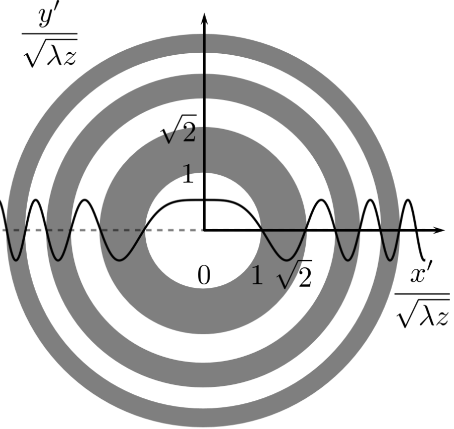
From bees to Vikings (see p. 51 in Optics f2f), from Harrison‘s chronometer to atomic clocks and GPS, navigation has always been a matter of live and death. Often, what begins as blue-skies scientific curiosity, may later save lives. A beautiful example is the work of Augustin-Jean Fresnel. One early success of Young’s experiments was to inspire Frensel to study shadows using a honey-drop lens in 1815. To explain his observations, Fresnel developed the theory of diffraction that we still use today, see Chapter 5 in Optics f2f. Fresnel’s experiments and theory firmly established the wave theory of light, and began a new way of thinking about optical devices such as the humble lens. For Fresnel, a lens was less about bending light, than ensuring that all parts of the wave arrive with their peaks and troughs synchronised (in phase) at the focus. Fresnel realised if we observe the light amplitude at a point then it is made up of contributions from the input plane that sometimes add in-phase and sometimes out-of-phase due to differences in the optical path. He separated the regions that add in and out-of phase into zones, where all the odd zones (white in the image below) have say a positive phase and all the even zones (grey in the image below) have a negative phase.
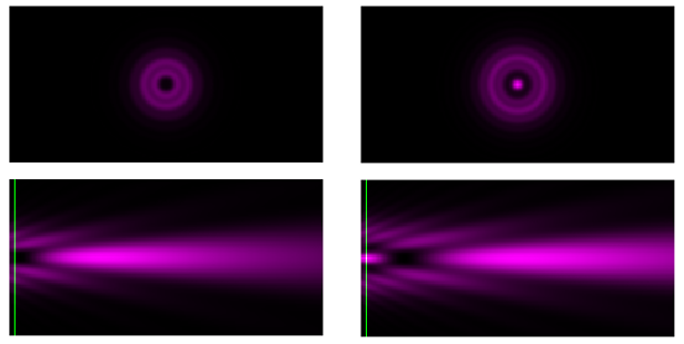
The white and grey regions contribute with positive and negative phase respectively and therefore interfere destructively with one another. He showed that the light contributions from neighbouring zones where equal and opposite. So if you use a circular aperture to block all the light except for the two central zones then you observe zero light intensity (on axis). If you increase the radius of the aperture to allow the third zone to contribute then you observe high intensity again. This is illustrated in the two images below which show the light intensity pattern downstream of a circular hole. In both cases, the top image is light intensity observed in particular plane and the bottom image is how the light distribution is changing as it propagates (the green line marks the observation plane). If you click on the interactive plot you can vary the diameter of the hole and see how the pattern changes. Note in particular how the observed intensity on-axis oscillates between zero and a maximum as more and more Fresnel zones are allowed to contribute.
Click here to see interactive figure.
Once you have this concept of Fresnel zones then you realise that to make all the light contribute with same (or nearly the same) phase you just need a small adjustment to the phase within each zones to make each contribution interference constructively at the focus. Consequently, to make a lens, instead of a big thick piece of glass we can use segments of glass that produce the desired phase shift for each zone. This idea, illustrated on the right below, is known as the Fresnel lens.
The Fresnel lens completely revolutionised lighthouse design as now it was possible to make much larger lenses constructed from smaller lighter segments. The first Fresnel lens was installed in the Cordouan lighthouse only 8 years after Frensel began his blue-skies experiment using a honey-drop lens. Postscript: The lighhouse story continues with another giant of nineteenth century physics, Michael Faraday. If you have the chance, go and visit his workshop below the Trinity Buoy Lighthouse in London.
Fraunhofer diffraction: experiment
Topics: N slit diffraction. Theory vs. Expt.
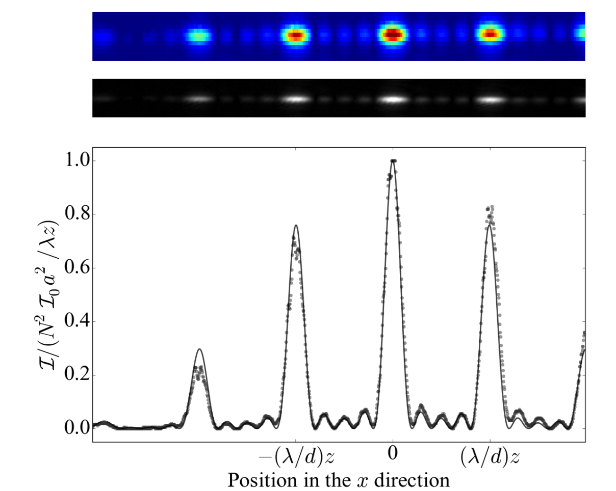
The gold standard of the scientific method is experiment (data) and theory on the same graph. Odd then that many optics textbooks show lots of theory curves and photos of interference or diffraction but rarely both ‘on the same graph’. This article discusses a simple example where we take a photo of a diffraction pattern and compare it to the prediction of Fraunhofer diffraction theory (see p. 85 in Optics f2f). All you need is a light source, a diffracting obstacle, and a camera. However, the trade-off is that to make the theory easier you need a more `idealised’ experiment. First, we show a photo of the far-field diffraction pattern recorded on a camera when an obstacle consisting of 5 slits is illuminated by a laser.
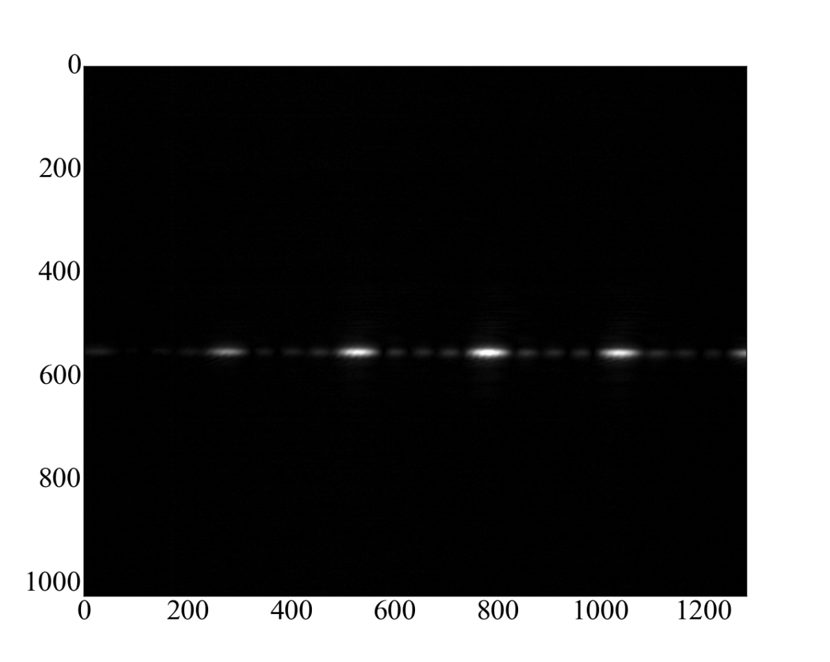
The experiment was performed by Sarah Bunton an Ogden Trust Intern at Durham in 2016. The image is in black and white and saved as a .png file. The image is read using the python imread command and ‘replotted’ with axes.
from numpy import shape, arange, sin, pi
from matplotlib import rc
rc('font',**{'family':'serif','serif':['Times New Roman']})
from matplotlib.pyplot import close, figure, show, pcolormesh, xlabel, ylabel, rcParams,  cm
from matplotlib.image import imread

fs=32
params={'axes.labelsize':fs,'xtick.labelsize':fs,'ytick.labelsize':fs,'figure.figsize':(12.8,10.24)}
rcParams.update(params)

img=imread('C:\Users\...\N_slits_5.png')
[ypix, xpix]=shape(img) # find size of image

close("all")
fig = figure(1,facecolor='white')
ax = fig.add_axes([0.15, 0.3, 0.8, 1.0])
ax.axison = False # Start with True to find region of interest
ax.imshow(img[500:600,:],cmap=cm.gray) #Show region

small=img.reshape([ypix/4, 4, xpix/4, 4]).mean(3).mean(1) # create super pixels
ax = fig.add_axes([0.15, 0.875, 0.8, 0.1])
ax.axison = False
ax.pcolormesh(small) #plot image of super pixels
ax.set_xlim(0,xpix/4)
ax.set_ylim(138-6,138+6)

cut=557 #Select horizontal line to compare to theory
data=img[cut,:]
data=data**1.5 #Gamma correction

ax = fig.add_axes([0.15, 0.1, 0.8, 0.6])
ax.axison = True
p=ax.plot(data,'.',markersize=10,color=[0.2,0.2,0.2],alpha=0.5)
ax.set_xlim(0,xpix)
ax.set_ylim(-0.05,1.05)

x=arange(0.0001,xpix,1.0) # x values for theory line
xoff=780
xd=x-xoff
flamd=252/(pi)
env=3.5*flamd
y=1.0*sin(xd/env)/(xd/env)*sin(5*xd/flamd)/(5*sin(xd/flamd))
y=y*y
p=ax.plot(x,y,linewidth=2,color=[0.0,0.0,0.0],alpha=0.75)
xlabel('Position in the $x$ direction')
ylabel('${\cal I}/(N^2{\cal I}_0a^2/\lambda z)$')
ax.set_xticks([xoff-pi*flamd, xoff,(xoff+pi*flamd)])
ax.set_xticklabels(['$-(\lambda/d)z$', '0','$(\lambda/d)z$'])

show()
Second, we select a row through the intensity maximum (lines 27-35) so that we can compare the intensity along the horizontal axis with the prediction of theory. For the theory (lines 37-48), we can measure the distances in the experiment (slit width, separation, distance to detector, pixel size and laser wavelength) or we can fit the data. Here we have only done a by-eye `fit’.
One thing you might notice in the code (line 29) is that we need to perform a scaling for the Gamma correction used by the camera. Some cameras may allow you to turn this off, otherwise you need to correct it in post-processing.
Young’s double: with colour
Topics: Interferometry, white light, coherence
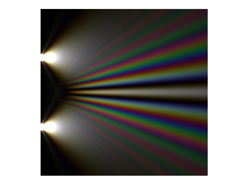
‘Young’s double slit’ has become the standard paradigm to explore two-path interference (Young actually did a very different experiment that requires a different explanation [1]). In the far-field, the ‘classic’ two-slit experiment produces fringes whose spacing is inversely proportional to the slit spacing. You can see this by varying the slit separation in the interactive figure linked below (credit to Nikola Sibalic).
Click here to see interactive figure.
Most textbooks only tell us about the far field, where the effect of diffraction dominates over the transverse size of the light distribution and we can make the Fraunhofer approximation, see e.g. p. 39 in Optics f2f. But now using computers it is easy to calculate the field everywhere. The code below uses Fresnel integrals, see p. 85 in Optics f2f, but we could also perform the calculation using Fourier methods, p. 99 in Optics f2f.
from numpy import dstack, linspace, size, sqrt, pi, clip, meshgrid
from pyplot import
from scipy.special import fresnel
from matplotlib.pyplot import close, figure, clf, show, imshow

Z, X = meshgrid(linspace(1,10001,480), linspace(-120,120,480))
R=0*X #initialise RGB arrays
G=0*X
B=0*X

wavelengths=linspace(0.4, 0.675, 12) # define 12 wavelengths + RGB conversion
rw=[0.1, 0.05, 0.0, 0.0,   0.0,   0.0, 0.0, 0.1, 0.13, 0.2, 0.2, 0.05]
gw=[0.0,  0.0,   0.0, 0.067, 0.133, 0.2, 0.2, 0.1, 0.067, 0.0, 0.0, 0.0]
bw=[0.1, 0.15, 0.2, 0.133, 0.067, 0.0, 0.0, 0.0,  0.0,   0.0, 0.0, 0.0]

a=12.5 #slit half width
off1=25.0 #slit offset

for ii in range (0,12): #add intensity patterns into the RGB channels
    l=wavelengths[ii]
    SA=a/sqrt(l*Z/pi)
    SX=X/sqrt(l*Z/pi)
    SOFF1=off1/sqrt(l*Z/pi)
    C1_2=fresnel(SA/2-SOFF1-SX)[0]-fresnel(-SA/2-SOFF1-SX)[0]
    S1_2=fresnel(SA/2-SOFF1-SX)[1]-fresnel(-SA/2-SOFF1-SX)[1]
    C3_4=fresnel(SA/2+SOFF1-SX)[0]-fresnel(-SA/2+SOFF1-SX)[0]
    S3_4=fresnel(SA/2+SOFF1-SX)[1]-fresnel(-SA/2+SOFF1-SX)[1]
    Intensity=0.5*((C1_2+C3_4)*(C1_2+C3_4)+(S1_2+S3_4)*(S1_2+S3_4))
    R+=rw[ii]*Intensity
    G+=gw[ii]*Intensity
    B+=bw[ii]*Intensity

brightness=4.0 #saturate
R=clip(brightness*R,0.0,1.0)
G=clip(brightness*G,0.0,1.0)
B=clip(brightness*B,0.0,1.0)
RGB=dstack((R, G, B))

close("all")
fig = figure(1,facecolor='white')
clf()
ax = fig.add_axes([0.05, 0.05, 0.9, 0.9])
ax.imshow(RGB)
ax.axison = False
show()
The code is so fast that it is easy to simulate white light using for example the 12 colour spectrum we introduced in Chapter 3. By modifying the spectrum light it is possible to explore coherence, see Chapter 8 in Optics f2f. By reducing the range of wavelengths, e.g. using a green filter as in the image below (in the code above, take the wavelength index from 4 to 8 instead of 0 to 12), we see higher fringe visibility off axis, see also Fig. 8.15 in Optics f2f, and we say that the light is more coherent.
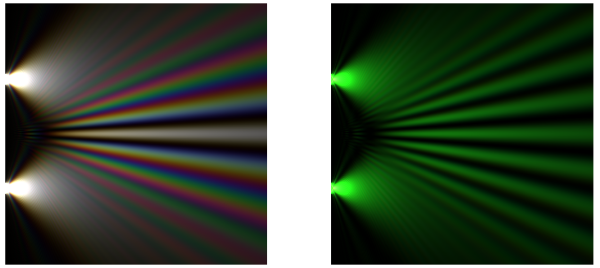
Click here to see interactive figure. The interactive plot provides a full colour version of Fig. 8.15 on p. 145 of Optics f2f
Young’s double slit using sunlight
What do we actually see if we do Young’s double slit experiment with white light, e.g. sunlight? The image below shows a picture of a double slit positioned in front of a camera with the camera looking towards the sun.
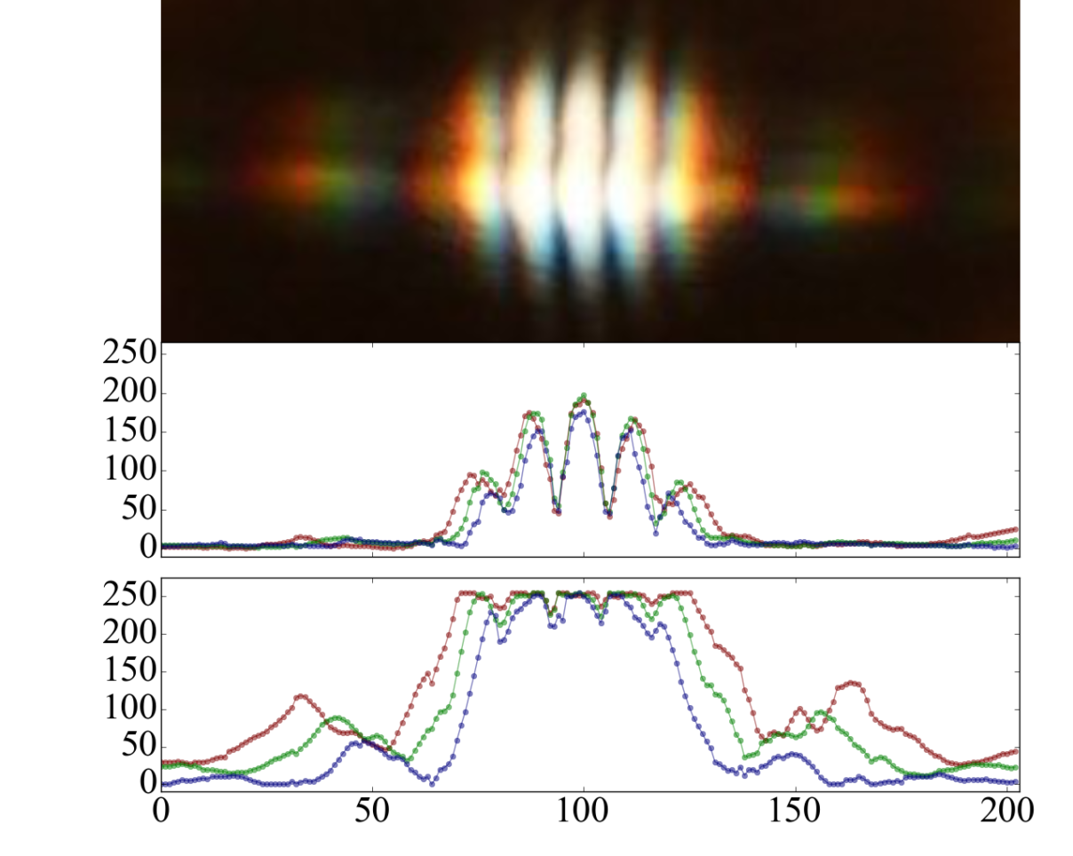
This is much more difficult to analyse unless we know how the exact spectral response of the RGB filters used in the camera, but still you can see some fun stuff like red is diffracted more than blue! Below is the code used to make this plot. Note on the imread command. If the image is colour then the data array may have three or four layers (RGB + tranparency) as well as horizontal and vertical position. In this example where we read in a jpg, direct from a camera.
from numpy import shape
from matplotlib import rc
rc('font',**{'family':'serif','serif':['Times New Roman']})
from matplotlib.pyplot import close, figure, show, rcParams,  cm
from matplotlib.image import imread

fs=32
params={'axes.labelsize':fs,'xtick.labelsize':fs,'ytick.labelsize':fs,'figure.figsize':(12.8,10.24)}
rcParams.update(params)

img=imread('C:\Users\...\young_sunlight.jpg')
[ypix, xpix, dim]=shape(img)

close("all")
fig = figure(1,facecolor='white')
ax = fig.add_axes([0.15, 0.3, 0.8, 1.0])
ax.imshow(img)
ax.axison = False

cut=40
data1=img[cut,:,0]-25
data2=img[cut,:,1]-10
data3=img[cut,:,2]

ms=10

ax = fig.add_axes([0.15, 0.35, 0.8, 0.25])
ax.axison = True
p=ax.plot(data1,'.',markersize=ms,color=[0.5,0.0,0.0],alpha=0.5)
p=ax.plot(data2,'.',markersize=ms,color=[0.0,0.5,0.0],alpha=0.5)
p=ax.plot(data3,'.',markersize=ms,color=[0.0,0.0,0.5],alpha=0.5)
p=ax.plot(data1,color=[0.5,0.0,0.0],alpha=0.5)
p=ax.plot(data2,color=[0.0,0.5,0.0],alpha=0.5)
p=ax.plot(data3,color=[0.0,0.0,0.5],alpha=0.5)
ax.set_xlim(0,xpix)
ax.set_ylim(-10,265)
ax.set_xticklabels([])

ax = fig.add_axes([0.15, 0.075, 0.8, 0.25])
ax.axison = True

cut=65
data1=img[cut,:,0]
data2=img[cut,:,1]
data3=img[cut,:,2]

ax.axison = True
p=ax.plot(data1,'.',markersize=ms,color=[0.5,0.0,0.0],alpha=0.5)
p=ax.plot(data2,'.',markersize=ms,color=[0.0,0.5,0.0],alpha=0.5)
p=ax.plot(data3,'.',markersize=ms,color=[0.0,0.0,0.5],alpha=0.5)
p=ax.plot(data1,color=[0.5,0.0,0.0],alpha=0.5)
p=ax.plot(data2,color=[0.0,0.5,0.0],alpha=0.5)
p=ax.plot(data3,color=[0.0,0.0,0.5],alpha=0.5)
ax.set_xlim(0,xpix)
ax.set_ylim(-10,275)

show()
[1] In his 1804 paper Young describes a experiment where a small hole is made in a screen to create a beam of sunlight. A thin card is placed in this beam to block the central portion such that the light can pass on either side and ‘interfere’ downstream: “I made a small hole in a window-shutter, and covered it with a piece of thick paper, which I perforated with a fine needle. For greater convenience of observation, I placed a small looking glass without the window-shutter, in such a position as to reflect the sun’s light, in a direction nearly horizontal, upon the opposite wall, and to cause the cone of diverging light to pass over a table, on which were several little screens of card-paper. I brought into the sunbeam a slip of card, about one-thirtieth of an inch in breadth, and observed its shadow, either on the wall, or on other cards held at different distances. Besides the fringes of colours on each side of the shadow, the shadow itself was divided by similar parallel fringes, of smaller dimensions, differing in number, according to the distance at which the shadow was observed, but leaving the middle of the shadow always white.” Such an arrangement is not easily explained by two-path interference. The diffraction pattern shown below is described by Fresnel diffraction in the near field and is a good example of Babinet‘s principle in the far-field, see p. 106 in Optics f2f.